

Analogy and Analog
First, a word about analogy. The word "analogy" comes from the Greek "analogia" ("αναλογια"), which combines the word "logion" with the prefix "ana". "Ana" is a kind of "double negative", while "logia" is either a feminine singular noun referring to a "science" or body of knowledge/sayings, or a neuter plural referring to many sayings. Used by itself today, the word normally applies to "a supposed collection of sayings of Jesus", but such words as "archaelogia" (science/body of knowledge about history) retain much their original meaning. A classic Greek would probably understand such words as "geologia" "meteorologia", etc. (The relationship between the feminine and neuter nouns is hardly accidental, it is present in many Indo-European languages and reflected in the identify of case inflection. An example from Latin is "casum"/"casa": the former referring to "room" the latter "rooms"/"house".)
In Greek, then, "analogia" would refer to representing one science or body of knowledge with another. More specifically, the word came to be used for "proportionality". In English, we use the broader sense of some system of identifying a particular subject in terms of another subject through similarities or parallels.
Early creation of analog computers used scalar quantities such as voltage to represent real-world scalars, while early digital computing machines replicated manual processes using "arabic" numberals. As the Stanford Encyclopedia of Philosophy points out:
As the case of the architect's model makes plain, analog representation may be discrete in nature (there is no such thing as a fractional number of windows). Among computer scientists, the term ‘analog’ is sometimes used narrowly, to indicate representation of one continuously-valued quantity by another (e.g., speed by voltage). [my emphasis]Similarly, from A Review of Analog Computing:
[... I]n a fundamental sense all computing is based on an analogy, that is, on a systematic relationship between the states and processes in the computer and those in the primary system. In a digital computer, the relationship is more abstract and complex than simple proportionality, but even so simple an analog computer as a slide rule goes beyond strict proportion (i.e., distance on the rule is proportional to the logarithm of the number). In both analog and digital computation—indeed in all computation—the relevant abstract mathematical structure of the problem is realized in the physical states and processes of the computer, but the realization may be more or less direct ([ref's]).We're going to use it in the narrow fashion.Therefore, despite the etymologies of the terms “analog” and “digital,” in modern usage the principal distinction between digital and analog computation is that the former operates on discrete representations in discrete steps, while the later operated on continuous representations by means of continuous processes ([ref's]). That is, the primary distinction resides in the topologies of the states and processes, and it would be more accurate to refer to discrete and continuous computation ([ref's]). [my emphasis]
Programming of Analog Computers
I've made analogies between the enzyme and gene activation systems, and analog computers created from networks of transistors and resistors, which are fairly "tight" in the sense that the voltage (or whatever, depending on specifics of design) is analogous to the concentration of enzyme or other factor. However, when we talk about "programming" analog computers, that draws an analogy to digital computers that is much looser.
What we know of as "programming" is pretty much a digital phenomenon. Let's back up to much simpler systems begin with: consider a digital system that samples its input (as discrete phenomena) and calculates an output, also discretely represented. This may be analogous to a network of transistors and resistors: each performs a pre-designed function and nothing else. Now expand the digital system to execute a "program" entered by setting switches on a board. These switches represent, in machine language, the steps the digital computer must follow to perform its activity. We may consider this analogous to a network of transistors and resistors with some potentiometers. twisting the knobs on the analog computer is equivalent to setting switches on the digital.
Now, digital computers will normally have memory of some type, registers to hold intermediate results, etc. But suppose some of this memory is used for its program: the program may be loaded into it just as switches are set manually, but the program itself may be data created through calculations. Finding an analogy to that with analog computers is much harder.
Instead, "programming" for analog computers normally refer(ed) to wiring.
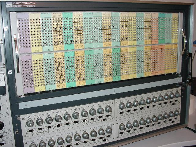
Figure 1: Hitachi 240: the patch panel above where "programming" takes place, below are the knobs which are used to enter input conditions, etc. (image from The HITACHI 240 Analog Computer by VAXMAN.)
There isn't really any analogy here with the enzyme system. If we regard the presence (or absence) of binding regions that react to specific transcription factors as analogous to patch cords in the panel of Figure 1, we might say that the total sequence of non-coding DNA "programs" the gene activation system, but even here the analogy is loose because there are many possible sequences for any binding region, with different "strengths" of affinity for TF's. Instead, we will consider the non-coding sequences (and such protein-coding sequences as perform dual functions) as "programming" but not try to make analogies with the patch cord system. Thus, we have no good electronic analogy for "programming" in the gene activation system.
In a general sense, the interactions between enzymes and DNA or other enzymes are "built in". This is because they have a "key/lock" interaction, which has no relationship to the amino-acid sequence that can be manipulated. Changes to the sequence are essentially random "shots in the dark" with results that have to be evaluated by Darwinian selection. There may be a partial exception regarding some DNA recognition regions where there is a predictable relationship between amino acid sequence and DNA base sequence, but we won't go into this here.
To discover something analogous to "programming" for the enzyme activation system, we have to take a closer look at the way catalysts work. This will also bring in the other elements of our title: power and speed.
A Word about Catalysis
When the catalyst amount is small, the reaction rate increases about linearly with substrate concentration. For our purposes, both the catalyst and the substrate are enzymes present in very small amounts. Thus the rate will almost always fall into region A in Figure 2:

Figure 2: Plot of substrate concentration vs. reaction rate (from the Medical Biochemistry Page).
Similarly, the rate will vary about linearly with catalyst amount.
Note that we usually aren't talking here about a reaction at chemical equilibrium. The energy of both phosphorylation and dephosphorylation is such that each reaction will proceed until the equilibrium ratio is in the neighborhood of 10,000:1. Thus the ratio of phosphorylated target enzyme to unphosphorylated will depend primarily on the relative rates, which in turn depend on the concentrations of kinases and phosphatases.
Enzymes Making a Basic Calculation
Let's take a simple example. We'll look at an enzyme we'll call Es, our substrate enzyme. (We'll assume linear responses here, which is usually a good approximation, although not exact.) Its output will be the absolute concentration of EsP, the phospho-activated form. The dephosphorylized form will be called Es0 (the zero for no phosphate). For simplicity's sake, we'll have two inputs, treated as absolute concentrations: Ek, the kinase that activates our substrate, and Ep, the phosphatase that deactivates it.
Start with 50% phosphorylation:
1×Ek + 1×Ep = 50% EsP, 50% Es0
That is, the amounts of kinase and phosphatase are balanced so the amounts of active and inactive substrate are equal. Now, if we double the amount of kinase, we double the ratio of active to inactive substrate:
2×Ek + 1×Ep = 67% EsP, 33% Es0
If we double the amount of phosphatase as well, we return the ratio to equal:
2×Ek + 2×Ep = 50% EsP, 50% Es0
Thus, in this simple case, we see that the absolute concentrations of the input enzymes don't matter, just the relative concentrations among the inputs.
Turning the Enzyme Knob
What happens if we go back to the beginning then add a whole bunch of new substrate, from a newly expressed gene?
*1×Ek + 1×Ep = 25% EsP, 75% Es0
I've put an asteroid beside the line, because it's out of balance: we just doubled the total amount EsP+Es0 by adding as much Es0 as the previous total. Since the rate of each reaction depends on both the concentration of its enzyme (unchanged) and that of its substrate (tripled for Es0), the rate of activation will be tripled compared to the rate of deactivation, and the ratios will quickly return to equal:
*1×Ek + 1×Ep = 25% EsP, 75% Es0
=== quickly ===>
1×Ek + 1×Ep = 50% EsP, 50% Es0
As you can see, the fraction of substrate that's activated remains constant for constant inputs (subject to settling time), however the absolute concentration has just doubled! To make it clearer, let's do it with absolute concentrations of Es: We start with 10 units of Es, divided equally:
1×Ek + 1×Ep = 5×EsP, 5×Es0
We add 10 more units of Es0:
*1×Ek + 1×Ep = 5×EsP, 15×Es0
=== quickly ===>
1×Ek + 1×Ep = 10×EsP, 10×Es0
As you can see increasing the total amount of our substrate enzyme is analogous to "turning up the gain" on an electronic amplifier", or twisting the knob on the potentiometer in our transistor network. The same input creates a stronger output.
In summary, then, the enzyme activation system can be "programmed" by the gene system, by increasing (or decreasing) the rate of gene expression for any specific substrate enzyme.
Programming of the Gene Activation System
What about the "programming" of the gene system I mentioned earlier? Well, the gene activation system is run primarily by the binding sites: their location and specific binding energies for each transcription factor. Since this is the result of mutation, as filtered through Darwinian selection, we can say that evolution has programmed the gene activation system.
Power and Speed
We saw, above, that increasing all the inputs by the same amount would leave the output the same (to a first approximation), while increasing the total substrate would increase the output (roughly) proportionally. So, in principle, couldn't we increase the concentration of all the enzymes in the system and have the same result?
Yes (sort of), but...
There are several factors involved here besides the actual answer to a calculation. Note that each time a molecule of substrate is activated, one molecule of ATP is hydrolyzed to ADP. Since the rates of activation and deactivation are equal (subject to a settling time labeled "quickly" in the above equations), one molecule of EsP is also hydrolyzed to Es0 + Pi (inorganic phosphate). If we double the total amount of substrate (Es), we double the amount of ATP being "burned" by the calculation.
So wouldn't it be better to keep the concentrations as low as possible? Yes, within limits. Let's go back to our original example:
1×Ek + 1×Ep = 50% EsP, 50% Es0
and reduce the inputs to 1/100th their previous:
0.01×Ek + 0.01×Ep = 50% EsP, 50% Es0
It looks like the same calculation, but what happens if we double the amount of kinase:
*0.02×Ek + 0.01×Ep = 50% EsP, 50% Es0
=== slowly ===>
0.02×Ek + 0.01×Ep = 67% EsP, 33% Es0
The settling time has been increased by 100, the speed reduced by the same factor. Thus, you can have smart, or you can have fast, but to have both you've got to spend a lot of energy. Another problem is random variation in quantities: Gene expression is roughly continuous, but if you reduce the concentrations enough you get enough noise in the system to be a problem. (Nature, Nurture, or Chance: Stochastic Gene Expression and Its Consequences by Arjun Raj and Alexander van Oudenaarden provides a recent review of noise in gene expression.)
What's needed, then, is a balance: enough to keep noise from interfering with the calculations, but not enough to burn more ATP than necessary.
For real speed, however, a digital approach can save a lot of energy. Here, the total concentrations of many enzymes in the system are high, but the activated forms of many are kept at very low relative concentrations. The system stays in a stable state until some external event triggers a positive feedback process that very quickly switches state. Once the new state has been achieved, either all the activated enzymes have either been reduced to very low concentrations, or their substrates have.
Is there trade-off in the gene activation system corresponding to the one described above for enzymes? Yes. The cost of transcribing RNA is two ATP's per base unit, as is the cost of adding each amino acid residue to a protein. (This is made clear in any biochemistry textbook, but I haven't found a good on-line reference for it.) The level of any protein can be maintained through continuous creation, overcoming the garbage disposal system, with a relatively low cost. However, when a gene has to be expressed at large levels, there has to be a dedicated disposal system for its protein. This can be either continuously maintained, or driven by part of the dynamic control system. Maintaining large amounts of transcription factors and high expression rates would also be expensive for the cell, and generally only happen for a few at a time, if that.
Are the concentrations of enzymes the same throughout the cell? Not always. In Part II I mentioned nuclear localization of transcription factors, but there's much more than that, the subject of the next post in this series.
Next How Smart is the Cell? Part IV: Local Intelligence
Links: (These include all the papers I used in creating this article, including the basics for many calculations not included here. I made them only to assure myself that I wasn't talking out my hat.)
The Modern History of Computing from Stanford Encyclopedia of Philosophy
A great disappearing act: the electronic analogue computer by Chris Bissell
A Review of Analog Computing Technical Report UT-CS-07-6 by Bruce J. MacLennan
Biochemical Energetics from Biochemistry of Metabolism
Enzyme Kinetics from the Medical Biochemistry Page
The Computational Versatility of Proteomic Signaling Networks
Sniffers, buzzers, toggles and blinkers: dynamics of regulatory and signaling pathways in the cell
Quantitative analysis of signaling networks
Coupled positive and negative feedback circuits form an essential building block of cellular signaling pathways
The Contents of Adenine Nucleotides, Phosphagens and some Glycolytic Intermediates in Resting Muscles from Vertebrates and Invertebrates by ISIDOROS BEIS and ERIC A. NEWSHOLME.
Roles of the creatine kinase system and myoglobin in maintaining energetic state in the working heart by Fan Wu and Daniel A Beard.
No comments:
Post a Comment